Post 1: Add ATAA Into UE4 -

The original paper adaptive temporal antialiasing by Adam Marrs et al. introduced how ATAA can be implemented with RTX in a summary. In this post, the focus is on the technique and problems I came across when adding ATAA to UE4 in a course project without RTX.

Segmentation

The first step to implement ATAA is to classify pixel types and record history information. In the paper, the pixel types include: FXAA, TAA, ATAA. The relevant information is a tracing counter to avoid jittering if a pixel switches between TAA and ATAA frequently. One render target was used to record them in R and G channels, respectively. Channel B records the luminance variance. Besides, I also recorded a TAA artifact level (TAL) in channel A, which is the sum of luminance variance and the gradient magnitude of $3 \times 3$ Sobel filter of depth texture. The higher this value is, the more artifacts TAA might produce. This value is stored for debugging and TAL visualization.

There are two interesting problems encountered in the way to generate the segmentation texture.

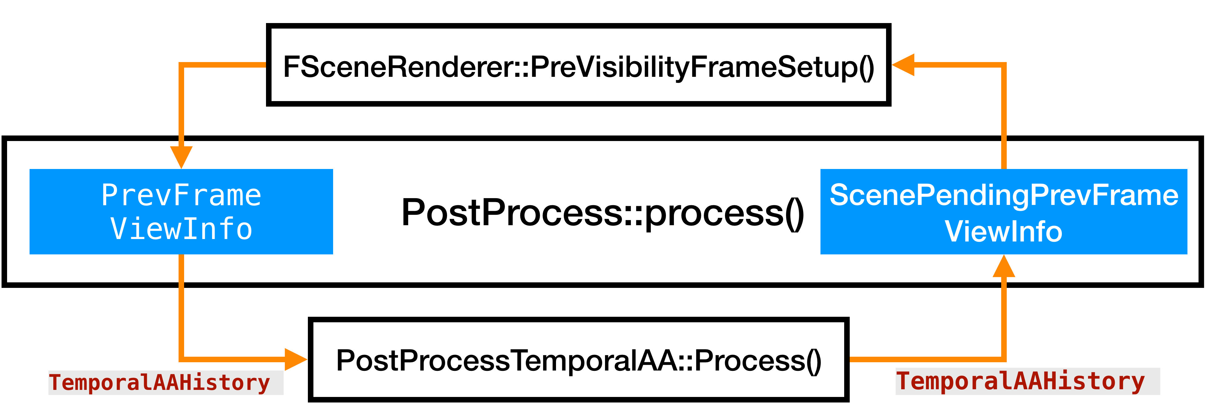
How to pass the segmentation texture between frames. We can add the render target into any place that survives between frames. But a clean code is preferred in a large code base like UE4. Since segmentation texture can be updated in PostProcessTemporalAA, we can make use of how UE4 passes TAA history between frames to achieve this. After exploring the code base, I found TemporalAAHistory could serve this purpose. The lifecycle is shown in image a) as below:


a) Lifecycle of `TemporalAAHistory`.	b) Variance comparison (gist)

This field is updated every frame from the ScenePendingPrevFrameViewInfo to PrevFrameViewInfo inside PreVisibilityFrameSetup.

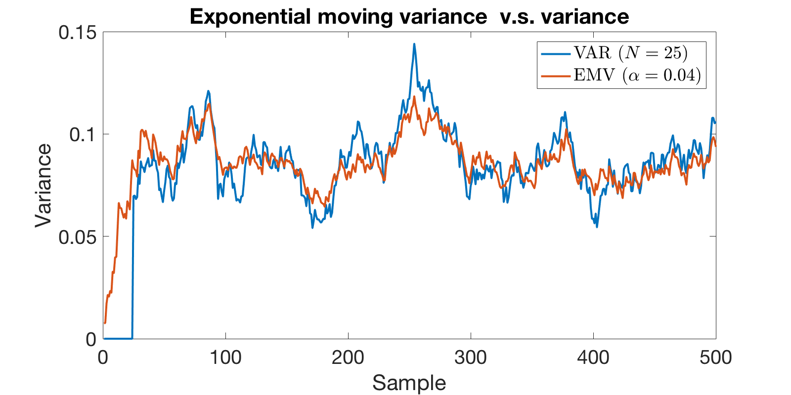
Luminance variance. The naive solution is to record the luminance for N frames and apply the variance formula as $$ V(X)=\frac{1}{N-1}\sum_{i=1}^N(x_i-\mu)^2 $$ However, this would require us to keep all $N$ render targets between frames, which is not economical. A better solution is one that we can update the variance online incrementally every frame. This is how TAA updates the pixel color of final rendering by applying exponential moving average. With the same idea, we can apply exponential moving variance (EMV) to achieve this as: $$ \mu_n = (1-\alpha) \mu_{n-1} + \alpha x_n $$ $$ \sigma^2_n=(1-\alpha)\sigma^2_{n-1}+\alpha(1-\alpha)(x_n-\mu_{n-1})^2 $$ where $\mu_n $ and $\sigma^2_n$ are the current exponential moving average and variance. $\alpha$ is the exponential weight. To illustrate whether EMV is suitable for this purpose, I applied both EMV and Variance to a 1D random signal, the result wqs shown in image b) above. It showed a high similarity between these two signals after code start.

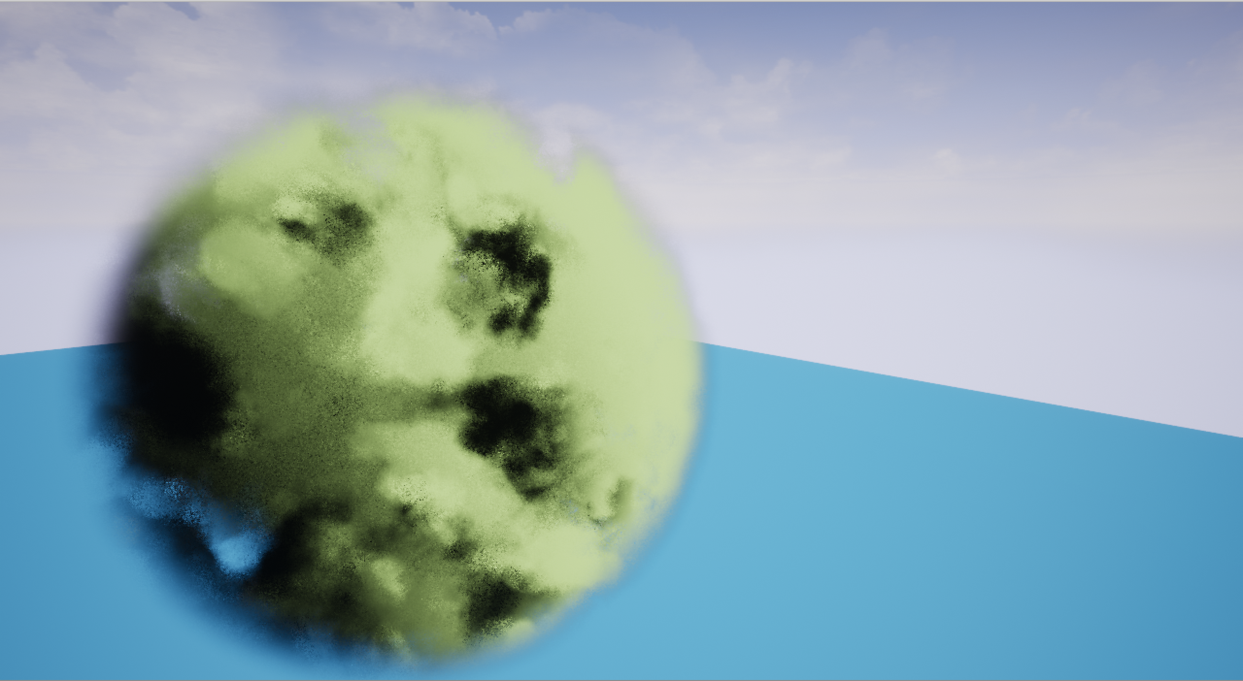
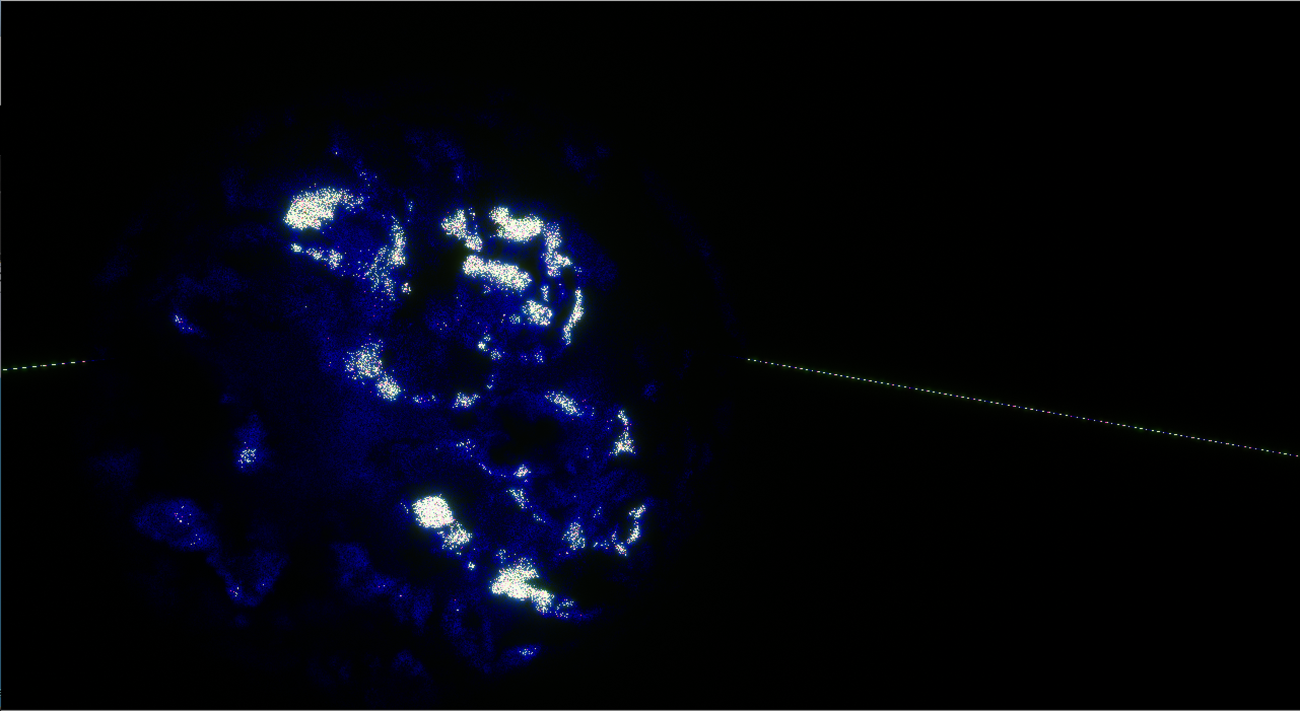
The image below shows a test scene and the corresponding segmentation texture. We can observe clear TAL as blue pixels especially for the volume object (You can open the image in a new window to see the detail).


Test Scene, a volume object above floor	The segmentation render target

The pseudo algorithm used in the project is as below:

0     //Assume that P holds all the property of the current pixel.
1     if(PreviousOccluded(P.Position,P.Motion))
2     {
3         P.ClassificationHistory.Method = FXAA;
4         return;
5     }
6
7     //Reset classification method.
8     if(SignificatMotion(P.Motion))
9     {
10        P.ClassificationHistory.Method = FXAA;
11        P.Classificationhistory.TracingCount = 0;
12        return;
13    }
14
15    //Whether the curent pixel has recently been traced.
16    //It reduces flickering due to rapid shifts with motion.
17    if(P.ClassificationHistory.Method == ATAA &&
18        P.ClassificationHistory.TracingCount-->0)
19    {
20        return;// because the method is ATAA
21    }
22
23    float TemporalLumiVar = GetTemporalLuminanceVariance();
24    float DepthMagnitude = Get3x3DepthMagnitudeWithSobel();
25
26    if(TemporalLumiVar+DepthMagnitude>Threashold)
27    {
28        P.ClassificationHistory.Method = ATAA;
29        P.ClassificationHistory.TracingCount = ConstTracingCount;
30    }
31    else
32    {
33        P.ClassificationHistory.Method = TAA;
34    }

A special note is that if there is a significant motion for a certain pixel, we will need to reset the method. If there is a significant motion, I would assume that the quality of the pixel is not important. Therefore, an early termination is triggered at line 12 to use FXAA (If the quality of significant motion is also important, line 12 can be removed).

Sparse Path Tracing

Instead of ray tracing with RTX as described in the original paper, a path tracer was created with compute shader to replace samples with high TAL. Because path tracing would reveal more dynamic details. The main challenge here is to have the same rendering result for both rendering pipelines: path tracing and rasterization based shading in UE4. Otherwise, the ATAA step itself will bring mismatch artifacts as shown below.


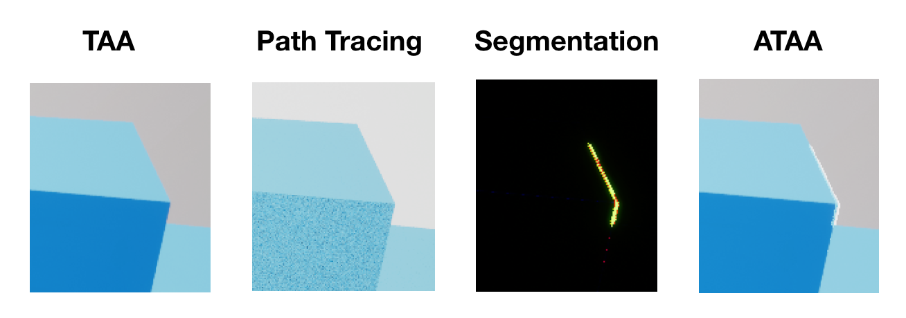ATAA brings in mismatch artifacts if path tracing and the rasterization result does not match.

Before solving this mismatch problem, let’s first see how the mismatch happened.

Iterative path tracer

Why an iterative path tracer: GPU is good at processing data in parallel in SIMD style by executing multiple threads at the same time (inside a warp on NVIDIA card). Yet it suffers from divergence problem caused by branches etc. Take branch as an example, if we have a path tracer executing recursively, it would create many different branching combination, yielding high divergence. If there is a ray that bounces 20 times while all others just once, all other threads need to wait for the single thread completion. After making it iterative, each pass will be independent. We can initialize 19 new rays to trace without the divergence brought in by recursive.

Another reason to choose an iterative path tracer for ATAA is to increase samples per pixel to reduce variance. Since samples to be traced are usually sparsely distributed. We need a way to only trace those pixels with high TAL. If it terminates early, we can sample the pixel again to reduce its variance.

Implementation: On each pixel that has high TAL value, a camera ray is initialized in the normalized device space (NDS) with a sub-pixel sampling pattern (i.e., Random and Sobol) and then transformed into the world space. Starting from the first interaction with the scene object, it incrementally samples path vertex by multiple importance sampling (MIS) of light and the BRDF at the current vertex and tracing a new ray to the next vertex until max bounce or termination by Russian roulette. If any ray has early termination, it will immediately fire another camera ray. At last, the results are averaged for each pixel.

I did not go for more advanced path tracing method like Bidirectional or Photon mapping. If you are familiar with the basic techniques, just ignore the following sections and jump to postprocess modification where the modification to add ATAA to the post process in UE4 is described.

Sub-pixel sampling

The purpose for sub-pixel sampling in rendering is to reduce visual impact of aliasing artifacts. Aliasing artifacts are introduced when sampling frequency is lower than twice the max frequency present in the signal based on Nyquist-Shannon sampling theorem. Those artifacts are the low frequencies leaked by high frequency signals (Interestingly, if we have a well-tuned high frequency image, we can see a different image if we are filming it with a camera that has an imperfect low pass filter).

Sub-pixel sampling can change the sampling pattern from uniform to nonuniform. Nonuniform sampling turns artifact pattern into random noise, thus reduces the visual impacts to our eye. However, we only need one sample per pixel for the final output. To achieve this, the high frequency was filtered out in the pixel region using Monte Carlo with filter kernel $\mathcal{F}(x_i,y_i)$, which ends up as: $$ f(x,y)_{filtered}=\frac{1}{N}\sum_{i=1}^{N}\frac{\mathcal{F}(x_i,y_i)\cdot f(x_i,y_i)}{p(x_i,y_i)} $$ where $f(x_i,y_i)$ is the sample result we get after path tracing at $(x_i,y_i)$. $p(x_i,y_i)$ is the probability density function that this coordinate is sampled. $\mathcal{F}(x_i,y_i) = 1$ if a box filter is applied inside the pixel region. However, to achieve higher filtering quality, other low pass 2D filter kernels can be applied (e.g., 2D Gaussian filter). If we further assume that the sampling is uniform, we have $p(x_i,y_i)=1$, which enables us to sample the filtered pixel as a weighted sum of all samples inside the pixel region.

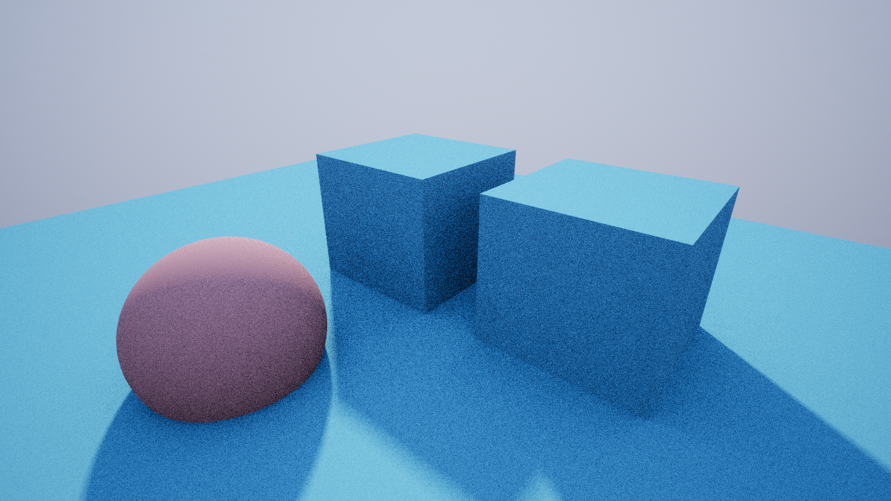
Result: I tried two different sampling patterns with uniform distribution including: random and Sobol sequence to generate 2D samples $(\varsigma_1, \varsigma_2) \in [0,1)^2$. The image below shows the comparison between a) random and c) Sobol sequence with sky irradiance only. Image b) is generated with 512 bounces as the baseline. We can observe clear edges with Sobol sequence as it will introduce known patterns. The edge is more smooth with random sampling.


Path tracing result with different sub-pixel sampling patterns. Early termination starts at the 4th bounce with Russian roulette. The sphere and box material was created with lambert BRDF. The only light in the scene is the sky irradiance which is represented as Order 3 Spherical harmonics.

However, sampling is not an end story here. Since we have limited sampling budgets for each pixel in real-time rendering, blue noise is a better method according to the frequency analysis course in SIGGRAPH Course 16’. In short, a homogeneous sampling strategy which has less spectral energy concentration on low frequency introduces less error for real-time rendering where we do not have enough samples. Blue noise samplers meet this requirement. So, it was chosen for BRDF sampling described in the next section.

BRDF sampling with limited budget

I only added Lambertian materials at this moment to support ATAA (to identify the difference between path tracing and rasterization). Lambertian materials have similar diffuse scattering radiance to all directions. In the incremental path tracing framework, Lambertian BRDF was used in the path throughput weight:

$$ \beta=\prod \frac{f(\omega_i,\omega_o)|n\cdot \omega_i|}{p(\omega_i,\omega_o)} $$

where $f(\omega_i,\omega_o)$ is the phase function, which is equal to $\frac{1}{\pi}$ for Lambertian. $p(\omega_i,\omega_o)$ is the probability distribution function. Since we have limited budget, cosine weighted sampling of BRDF is better than uniform, which makes $p(\omega_i,\omega_o)=\frac{1}{\pi}$. To have cosine weighted hemisphere sampling, a simple method without coordinate space transform is to add the surface norm to a random uniform vector sampled on a unit sphere. Since we cannot afford too much rays for this sampling, I went for the method that has the best convergence rate when sample count is low, which lead me to blue noise on unit sphere.

A little more about blue noise: There are several blogs about blue noise on 2D space. You can read more about it from demofox’s blog about Mitchell’s Best Candidate Algorithm and Christoph’s free blue noise texture. If you prefer generation speed, Pixal’s EGSR 18’ Paper is well worth reading.

Blue noise on unit sphere: To generate sample points on unit sphere, I chose the algorithm to generate points with best blue noise property offline and then upload an LUT to use in the shader. Mitchell’s best candidate algorithm was selected because the closest neighbor points have the largest distance based on Pixal’s EGSR paper. Moreover, it was generated progressively. The number of sampling points can be configured in the shader with only one LUT. Although SIGGRAPH Course 2016 suggested CCVT (Capacity constrained Voronoi Tessellation) as it has the best convergence rate, it was not used given the time limitation. The basic idea of Mitchell’s best candidate algorithm is that at each iteration keep the random generated candidate that is furthest to the closest points already selected in previous iterations . A special note for using this algorithm on sphere, instead of using Euclidean distance, the Great-circle distance should be used to calculate the closest distance between two points on the sphere. The vector version which is handy is listed here:

$$ d=arctan(\frac{|\mathbf{p}_1 \times \mathbf{p}_2|}{\mathbf{p_1}\cdot\mathbf{p}_2}) $$

which is the arctan of the magnitude of the cross product of the two points $\mathbf{p_1}$ and $\mathbf{p_2}$ by their dot product.

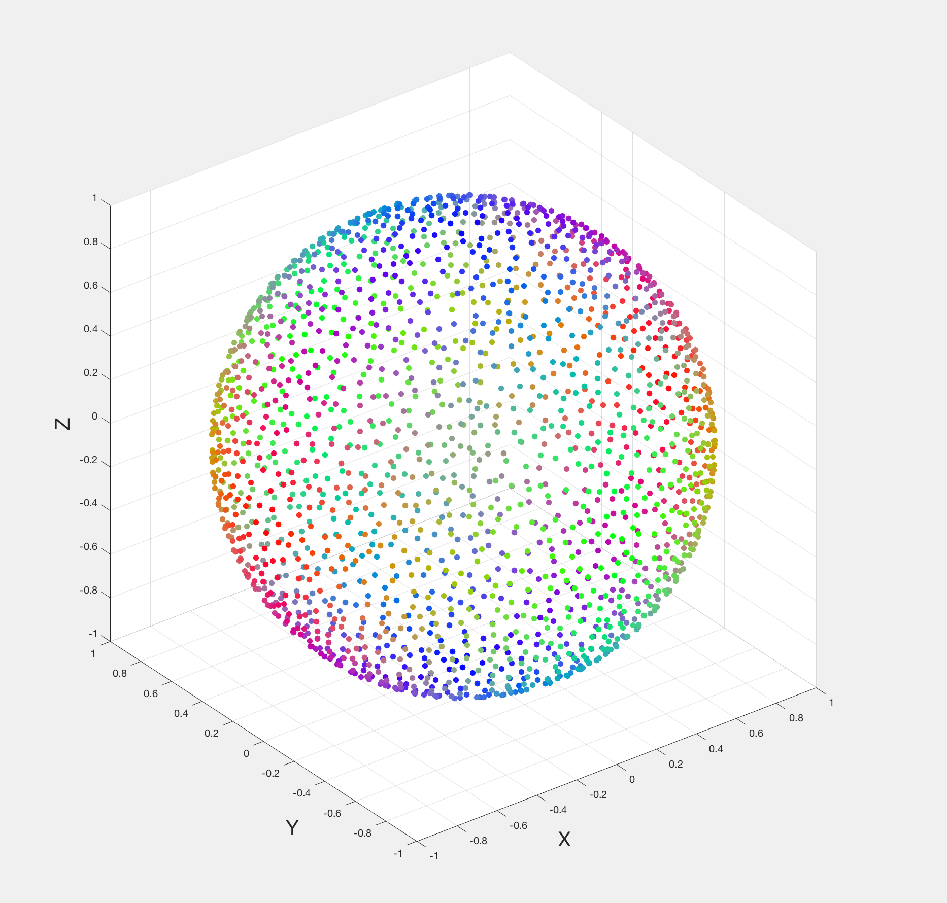
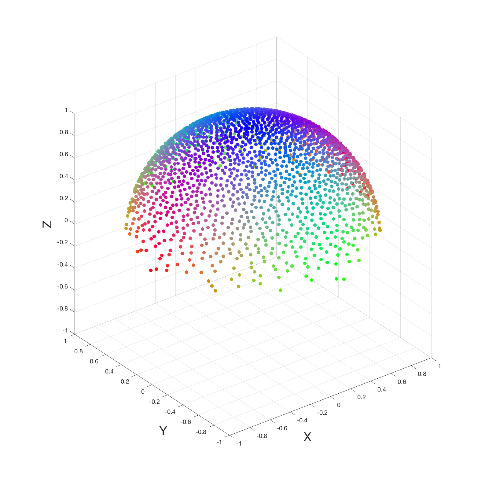
The image below shows sample generations a) when the number of points is 2048 with blue noise on sphere (gist), b) converted to cosine weighted sampling on hemisphere, c) looking down from Z Axis, and d) with random sampling and looking down from Z axis.


a) Blue noise sampling on unit sphere (N=2048)	b) Converted to cosine weighted sampling on hemisphere

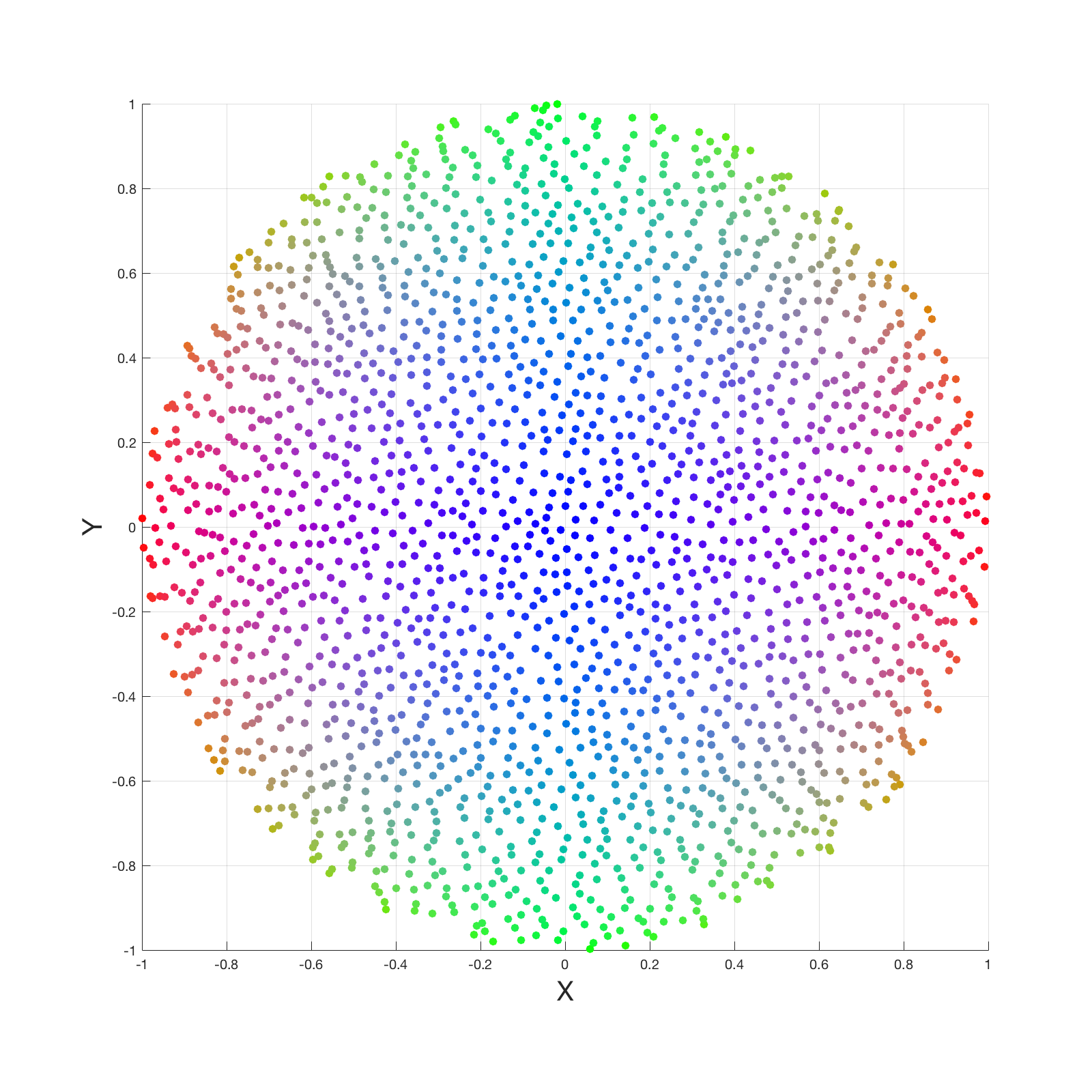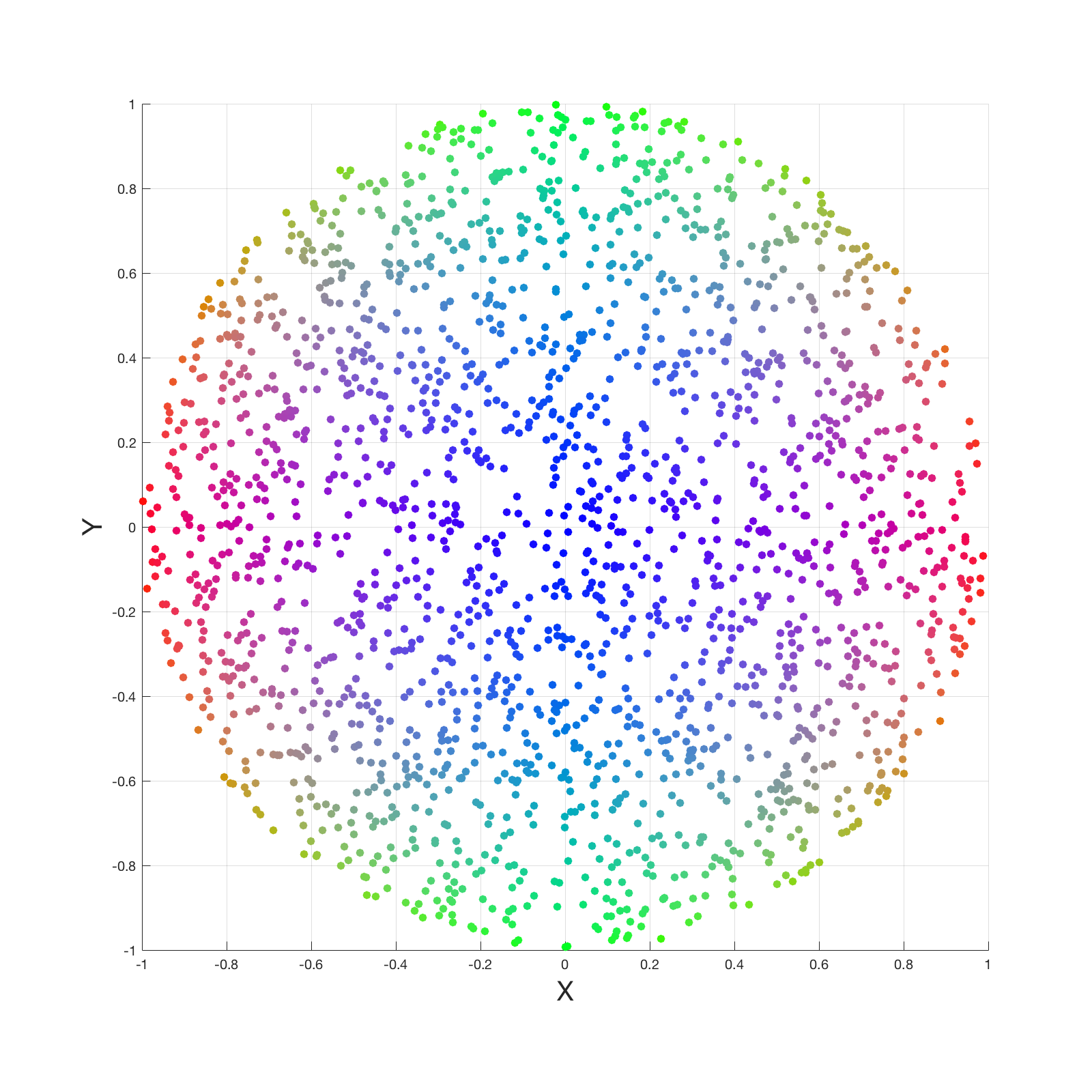c) Blue noise looking down from Z Axis	d) Random sampling looking down from Z Axis

It is clear that random sampling is clumpy. However, the blue noise can be better if we sample blue noise on a disk and then project it up onto a hemisphere. Nevertheless, I did not go this way. Because it requires an additional local coordinate construction and matrix multiplication at each interaction.

Result: Below are two frames captured when two different BRDF sampling method is used while other paramters are fixed. If we use blue noise sampling, it has less clumpy sampling points over all. Therefore, in brighter region, it converges to bright faster, and in dark region it converges to dark faster. In order to see which one converges better, I set the max bounce per ray to 1, and fixed the sub-pixel sampling method to Sobol Sequence and the total bounce to 256.


Random Sampling	Blue noise sampling

The difference is minute. Yet if you observe it closely (open them in another tab), you will find the top right region of the box is brighter in blue noise sampling, and the ambient occlusion of the sphere is darker for blue noise.

Multiple importance sampling of light and brdf

In the current implementation, I only added the sunlight in addition to the skylight. Because by default when you create an UE4 scene, there are sunlight and skylight in the scene. However, if we only sample the BRDF of the material, we can hardly see them with limited sample counts. To increase the efficiency of Monte Carlo integration, we can do multiple importance sampling that combines BRDF and light sampling.

To achieve this, we need to simplify the multi-sample estimator:

$$ F=\sum_{i=1}^n\frac{1}{n_i}\sum_{j=1}^{n_i}w_i(X_{i,j}) \frac{f(X_{i,j})}{p_i(X_{i,j})} $$

I have fixed the weighting function of both sampling strategy, and drawn one sample from each sampling technique, which simplified the importance sampling function as:

$$ F=w_1\frac{f(X_{1,1})}{p_1(X_{1,1})}+w_2\frac{f(X_{2,1})}{p_2(X_{2,1})} $$

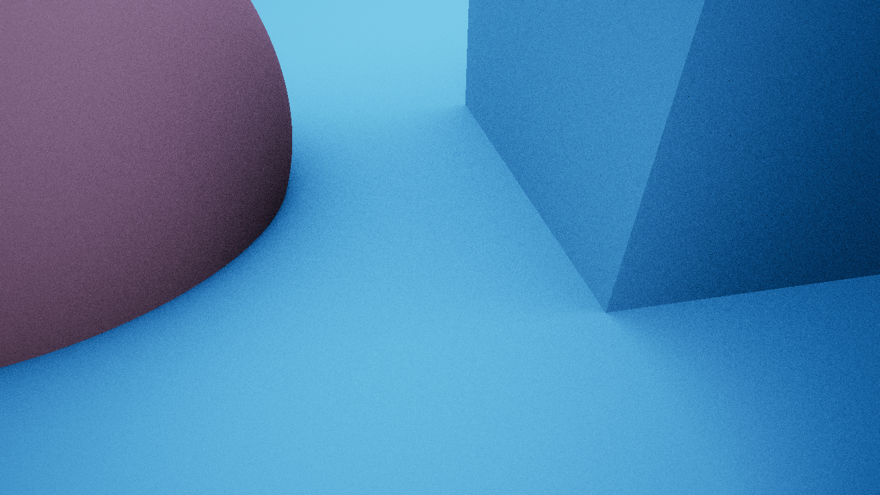
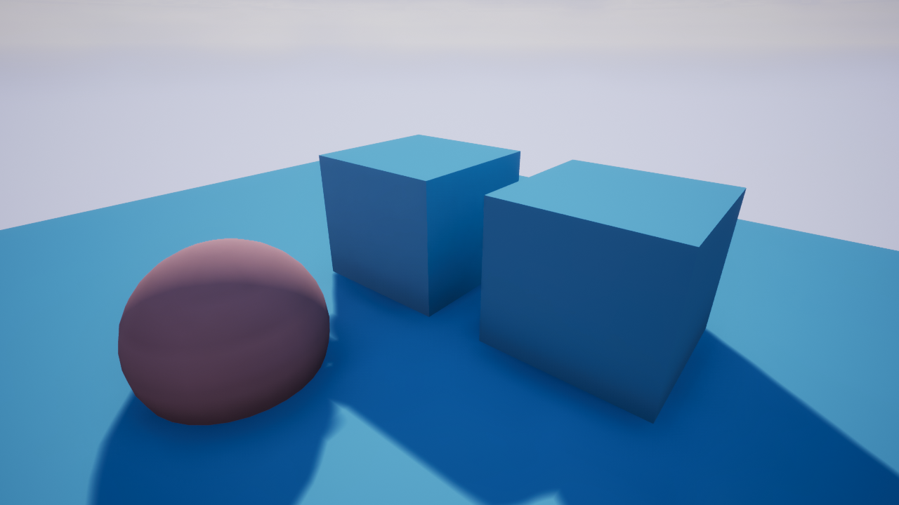
This combination will have high variance if the sunlight and BRDF sampling technique were bad. But I find it relatively good (I do not have too much experience about how good it can be with limited number of bounces). The image a) below shows the rendering result with random sub-pixel sampling and 64 bounce. Each ray can only bounce once, which is equal to 32 spp.


a) Importance sampling of sunlight and skylight	b) Default lighting in UE4

c) Randomize light ray to create PCSS	d) Soft shadow result for path tracing

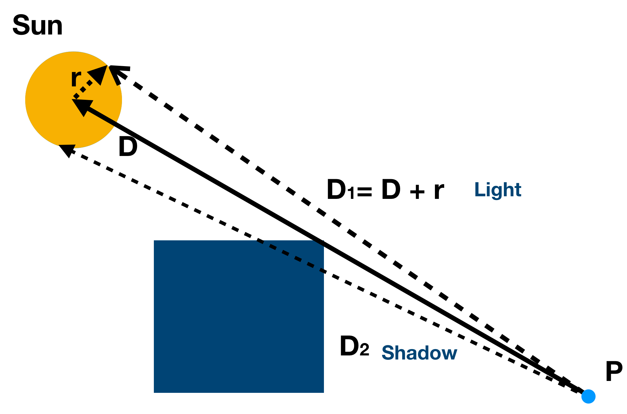
However, objects in UE4 cast soft shadows by default as shown in Image b) above. A cascading shadow map is used to generate softshadow. To add soft shadow in the path tracing framework, I randomized the light ray bouncing to the sun in the sun region (shown in Image c)). Then, in the next iteration, it will bounce to an obstacle if it cannot hit the sun, or into the sun to create lighting contribution. The final result is shown in image d). We can freely get percentage close soft shadow (PCSS). However, PCSS is costly in UE4.

If you compare the soft shadow only in image b) and d), you can notice two difference.

Jaggy difference. To the best of my knowledge, the jaggy shadow in UE4 is due to the cascading shadow map resolution. It seems that UE4 has a special correction for shadow if they are close to each other, as shown between the sphere and the box. Yet, I still need to figure out what that is.
Shadow Softness. The path tracing soft shadow by default has PCSS features. The shadow is sharper closer to the object and more blurry further to it.

So, this is all that we need to implement to apply ATAA to UE4 if we have tons of ray. However, there are still several difference we need to address before we can use ATAA in this simple situation. You can find more differences by comparing iamge b) and d). Yet I stopped here for the path tracing part.

Even with this, we can find a subset of features to apply ATAA, which will be detailed in applying ATAA to volume object rendering. In the next section, I will focus on how ATAA can be added to the post process pipeline in UE4 version 4.20.2 that I am using.

Postprocess modification

For basic postprocess pass editing, you can read Dr. Marc Olano’s course website for graphics for games taught at UMBC. It introduces all information you need to know about UE4 to implement techniques like ATAA into UE4 rendering pipeline.

1). Segmentation. I duplicated the FRCPassPostProcessTemporalAA class as ~Plus, and added an additional FRenderingCompositeOutput named Segmentation. In the pixel shader, the TemporalAASample function is called as usual. In addition, we need to record other information including:

Offscreen to indicate if there is no history. This pixel will use FXAA to denoise.
Velocity to de-noise fast moving pixels with FXAA.
ClassificationHistory from the last history render target, where the z component is the updated EMV value. w is the TAL value.
DepthMagSobol to indicate the depth neighbor variance of the pixel.

Those values will be collaboratively used to determine the segmentation texture.

2). Sparse path tracing. I duplicated the FRCPassPostProcessDownsample class as FRCPassPostProcessSparsePathTracing and registered it to the PostProcess graph after Bokeh pass, because it has compute shader templates, which is quite helpful for the implementation of the sparse path tracing. Then the path tracer mentioned above is implemented and traces pixels that only has high TAL. This post GPU Ray Tracing in One Weekend helps a lot for the implementation. However, there are three problems that I have run into:

I did not previously know that all view uniform variables are not accessible in Compute Shader by default even after setting the view uniform for the global shader. We need to add codes to support them. A lot of time was spent to find it out.
Since we need to generate the camera ray, we need to remove the TAA dithering when obtaining the inverse view matrix. In UE4, all related matrix is managed in ViewMatrices. You can either get it there or set the dithering entries to zero.
There is no explicit API to upload FRWBufferStructured arrays, which I used to upload the geometry and LUTs. But you can write your own encapsulation. This question Create structured buffer questions asked at UE4 forum is very helpful. To get the basic geometry shape, I added one public API to the FPrimitiveSceneInfo class to access the primitive component, which is originally designed for debugging. Because this is the only way I find to get material properties dynamically like Albedo.

3). Combine. Now that we have the sparsely traced pixel colors, we can combine it with the original TAA pixels. To achieve this, I add an ATAACombine pass to combine TAA and Sparse path tracing result just before Tonemaping. The reason to do it before this pass is that all color operation is in linear RGB space and passes after this point will be converted to sRGB space that considers human vision characteristics.

In this pass, the original pixel marked as ATAA is directly replaced by the corresponding path tracing color.

4). FXAA. The last modification is to modify the FXAA pass. We can directly apply FXAA to the pixel where it is marked as FXAA in the segmentation image. Because we have already combined ATAA and TAA image, and those pixels from TAA are sampled from the texture passed into TAA pass directly.

Future Work

Support volume objects. In this post, the supported material is only lambertian. To add volume objects that have the same behavior of UE4 can not be directly achieved by path tracing a volume. Because that will not have the same rendering result. Moreover, custom volume objects in UE4 do not have shadows, we need to ignore the volume objects that is hit after hitting an opaque surface in the tracer. At last, we need to correctly combine the volume objects that are transparent (The volume objects support is added in the next post).

Correct global illuminance. If you observe the rendering result closely, the color has some mismatch, especially the shadow region that only relies on global illuminance. The sky irradiance modeled by Order 3 Spherical Harmonics in UE4 was used for this purpose. However, it is more complex than I thought.

Divergence. Up till now, the sparse tracing is not well optimized. For each (8,8,1) thread group. The ATAA flag is test for each pixel. If only one pixel has high TAL, the other 63 threads are wasted waiting. Although the performance now is not bad, I can achieve an amortized rays of 7.1G Rays/s on GTX 1080 (327M Rays/s for full screen tracing), it can be improved further by aggregating ATAA pixels. I am still working on this.

Ray object intersection optimization. In the current implementation, each ray iterates all objects in the scene to find a hit. With more objects and detailed meshes, an acceleration structure (e.g., bounding volume hierarchy) is required to make it faster. Otherwise, we cannot use ATAA on all objects, we can only limit the application range to few material type, like volume objects only.

Helpful tips on Mac

Since the only working platform is macOS, I do not have the access to the great tool RenderDoc. If only it is already supported on Mac. So, two basic tools were used (Hopefully there are better tools existing):

Digital color meter on mac for debugging color output in sRGB space.
Create unit test case to test the alignment of structures on CPU and GPU for RWBufferStructured in shader. Otherwise, it was hard to align them, because my structure field was not 16 bytes aligned.